実験計画法（６）－グレコ・ラテン方格

実験計画法のうち、ラテン方格からさらに発展したグレコ・ラテン方格法について述べます。

グレコ・ラテン方格法

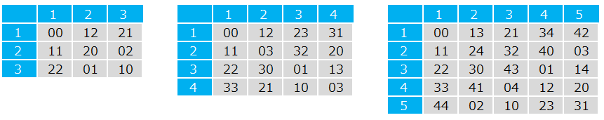
ラテン方格とはn行xn列の表にn個の異なる記号が各行各列に1度だけ現れる表です。このラテン方格の各記号に実験水準を割り当てる実験計画法がラテン方格法です。

表中の記号を2つに増やし、どの組み合わせも他と異なっている場合にグレコ・ラテン方格（またはオイラー方陣）と呼びます。つまり2種類のラテン方格の重ね合わせです。

グレコ・ラテンの名は数学者オイラーが、2つの記号にローマ字（ラテン文字, Latin）とギリシャ文字（Graeco）を用いたことに由来するそうです。

ラテン方格の場合と同様に、グレコ・ラテン方格は行、列、表中2記号から4要因の実験と捉えることが出来ます。

グレコ・ラテン方格を作れない場合

グレコ・ラテン方格はn=2とn=6の場合は作れません。n=2の場合のラテン方格は下記です。

これに対して2つめの記号を列挙すると下記の通り。

全てグレコ・ラテン方格の性質を満たすことが出来ません。

オイラーはこれを一般化して4m+2、つまりn=2,6,10,14,...ではグレコ・ラテン方格は作れないと予想しました。1961年にGaston Tarry[1]がn=6では作れないことを証明し、1960年代の研究でn=2,6以外でグレコ・ラテン方格が作成できることが証明されています[2][3][4][5]。

グレコ・ラテン方格法の分散分析

グレコ・ラテン方格でも、二元配置実験の場合と同じように、分散分析を行うことが出来ます。

総データ数を[math] N [/math]、水準数を[math] n [/math]、総和を[math] T [/math]、A条件[math] i [/math]水準の総和を[math] \displaystyle T_{ i \cdot \cdot \cdot} [/math]、B条件[math] j [/math]水準の総和を[math] \displaystyle T_{ \cdot j \cdot \cdot} [/math]、C条件[math] k [/math]水準の総和を[math] \displaystyle T_{ \cdot \cdot k \cdot} [/math]、D条件[math] l [/math]水準の総和を[math] \displaystyle T_{ \cdot \cdot \cdot l} [/math]とすると各平方和は下記の通り。

修正項　[math] \displaystyle CT = \frac{T^2}{N} [/math]
総平方和　[math] \displaystyle S_T = \sum_{i=1}^{N}{x_i}^2 - CT [/math]
A要因平方和　[math] \displaystyle S_A = \sum_{i=1}^{n} \frac{ {T_{ i \cdot \cdot \cdot }}^2}{ n^2 } - CT [/math]
B要因平方和　[math] \displaystyle S_B = \sum_{j=1}^{n} \frac{ {T_{ \cdot j \cdot \cdot }}^2}{ n^2 } - CT [/math]
C要因平方和　[math] \displaystyle S_C = \sum_{k=1}^{n} \frac{ {T_{ \cdot \cdot k \cdot}}^2}{ n^2 } - CT [/math]
D要因平方和　[math] \displaystyle S_D = \sum_{l=1}^{n} \frac{ {T_{ \cdot \cdot \cdot l}}^2}{ n^2 } - CT [/math]
誤差平方和　[math] \displaystyle S_E = S_T - S_A - S_B - S_C - S_D [/math]

各自由度は下記のようになり、

総自由度　[math] \displaystyle \phi_T = N - 1 [/math]
A要因自由度　[math] \displaystyle \phi_A = n - 1 [/math]
B要因自由度　[math] \displaystyle \phi_B = n - 1 [/math]
C要因自由度　[math] \displaystyle \phi_C = n - 1 [/math]
D要因自由度　[math] \displaystyle \phi_D = n - 1 [/math]
誤差自由度　[math] \displaystyle \phi_E = \phi_T - \phi_A - \phi_B - \phi_C - \phi_D = N - 4n + 3 = (n-3)(n-1) [/math]

一元配置実験と同様に下記のような分散分析表を作成できます。また上式より、n=3の場合は誤差分散が0のため有意差検定が出来ないことが分かります。

要因	平方和	自由度	平均平方	[math] \displaystyle F_0 [/math]値	[math] \displaystyle P [/math]値
A	[math] \displaystyle S_A [/math]	[math] \displaystyle \phi_A = n - 1 [/math]	[math] \displaystyle V_A [/math]	[math] \displaystyle {V_A}/{V_E} [/math]	[math] \displaystyle P_A [/math]
B	[math] \displaystyle S_B [/math]	[math] \displaystyle \phi_B = n - 1 [/math]	[math] \displaystyle V_B [/math]	[math] \displaystyle {V_B}/{V_E} [/math]	[math] \displaystyle P_B [/math]
C	[math] \displaystyle S_C [/math]	[math] \displaystyle \phi_C = n - 1 [/math]	[math] \displaystyle V_C [/math]	[math] \displaystyle {V_C}/{V_E} [/math]	[math] \displaystyle P_C [/math]
D	[math] \displaystyle S_D [/math]	[math] \displaystyle \phi_D = n - 1 [/math]	[math] \displaystyle V_D [/math]	[math] \displaystyle {V_D}/{V_E} [/math]	[math] \displaystyle P_D [/math]
E	[math] \displaystyle S_E [/math]	[math] \displaystyle \phi_E = N - 4n + 3 [/math]	[math] \displaystyle V_E [/math]
T	[math] \displaystyle S_T [/math]	[math] \displaystyle \phi_T = N - 1 [/math]

まとめ

ラテン方格と来たら、次はグレコ・ラテン方格です。実験計画法的な視点の他に、オイラーの業績と推測と後人による証明/反証に触れられて大変興味深いです。

[1]Tarry, Gaston (1900). "Le Problème Des 36 Officiers." Comptes Rendus Assoc. France, Av. Sci. 29, 170-203.
[2]Bose, R.C., Shrikhande, S.S. (1959). On the falsity of Euler’s conjecture about the non-existence of two orthogonal Latin squares of order 4t + 2. Proc. Nat. Acad. Sci. U.S.A. 45, 734–737.
[3]Parker, E.T. (1959). Construction of some sets of mutually orthogonal Latin squares. Proc. Amer. Math. Soc. 10, 946–949.
[4]Parker, E.T. (1959). Orthogonal Latin squares. Proc. Nat. Acad. Sci. U.S.A. 45, 859–862.
Bose, R.C., Shrikhande, S.S., Parker, E.T. (1960). Further results on the construction of mutually orthogonal [5]Latin squares and the falsity of Euler’s conjecture. Canadian J. Mathematics 12, 189–203.